SVM

Support Vector Machine

Notes:

• Please remember the below list of words in your mind before getting into the Session.
  1. hyper-plane.
  2. Margins.
  3. Support Vectors.
  4. Kernal.
  5. SVM = Support Vector Machine.
  6. SVR = Support Vector Regression

1. Introduction:

• Welcome to the 3'rd module of Classification models, Classifying data is a common task in machine learning. Suppose some given data points each belong to one of two classes, and the goal is to decide which class a new data point will be in. In the case we can go for Support-Vector Machines[SVM].
• A Support Vector Machine (SVM) is a discriminative classifier formally defined by a separating hyper-plane.
• In other words, for given labeled training data (supervised learning), the algorithm outputs an optimal hyper-plane which categorizes new data points.
• In two dimensional space this hyper-plane is a line dividing a plane in two parts where in each class lay in either side.
• SVM is another simple algorithm that every machine learning expert should have in his/her arsenal. and it is highly preferred by many as it produces significant accuracy with less computation power.
• SVM can be used for both regression, classification and outliers detection tasks. But, it is widely used in classification tasks.
• Keep in mind that, the objective of the support vector machine algorithm is to find a hyper-plane in an N-dimensional space[N — the number of features] that distinctly classifies the data points.

1.1 Advantages of SVM:

• Effective in high dimensional spaces.
• Still effective in cases where number of dimensions is greater than the number of samples.
• Uses a subset of training points in the decision function (called support vectors), so it is also memory efficient.
• Different Kernel functions can be specified as decision function.

1.2 Assumption:

• Suppose you are given plot of two label classes on graph as shown in below image(Fig-1). Can you decide a separating line for the classes? Note: here X and Y are considered as dimensions.

• You might have come up with something similar to below image(Fig-2). It fairly separates the two classes[For Assumpsion].

• Any point that is left of line falls into blue Plus class and on right falls into Orange Minus class.
• You may have a question here, What SVM is actually doing here, the answer to your question is Separation of classes. That’s what SVM does.
• It finds out a Optimal line/hyper-plane between two classes shown as below image(Fig-3)[Green line is the Optimal Hyper-plane].

2. Hyper-Plane: (Decision Boundary)

• Obj: As all we know the main role of Hyper-Plane is to distinctly classifies data-points as N-dimensional space with Maximum Margin.
• To separate the two classes of data points, there are many possible hyper-planes that could be chosen(Like shown above Fig-3), Our objective is to find a plane that has the maximum margin, i.e the maximum distance between data points of both classes to the Margin.
• Maximizing the margin distance provides some reinforcement so that future data points can be classified with more confidence.
• Hyper-planes are decision boundaries that help classify the data points. Data points falling on either side of the hyper-plane can be attributed to different classes.
• Most importantly the dimension of the hyper-plane depends upon the number of features.
• Example:
  • If the number of input features is 2, then the hyper-plane is just a line.
  • If the number of input features is 3, then the hyper-plane becomes a two-dimensional plane.
  • It becomes difficult to imagine when the number of features exceeds 3

Img Source: https://en.wikipedia.org/wiki/File:SVM_margin.png Author: Larhmam

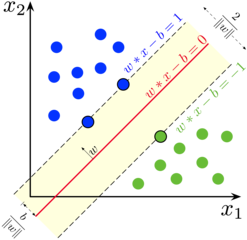
• In the above shown image,
  • The RED line with equation w*x-b=0 is considered as Boundary Line(Hyper-Plane).
  • The dashed Black line is considered as Margins or Boundary Margins or Maximum Margins(Will see more about margins in later topic).
  • The blue and Green dots where exactly placed on Buondary Margin are known as "Support Vectors"
  • Anything above the Margin (wx-b=1) are considered to be class 1 and anything below to the Margin (wx-b=-1) are considered to be Class -1.
  • So in our case we can assume Blue dots belongs to Class 1 and Gree dots belongs to Class -1
  • w --> normal vector to the hyperplane. This is much like Hesse normal form, except that w is not necessarily a unit vector.
  • x --> P-dimentional real vector
  • b --> constant

3. Support Vectors:

• Support vectors are data points that are closer to the hyper-plane and influence the position and orientation of the hyper-plane, Using these support vectors, we maximize the margin of the classifier.
• Deleting the support vectors will change the position of the hyper-plane. These are the points that help us build our SVM.

4. Parameter Tuning: Kernel, Regularization, Gamma and Margin:

4.1 Kernal:

• The learning of the hyper-plane in linear SVM is done by transforming the problem using some linear algebra. This is where the kernel plays role.
• For linear kernel the equation for prediction for a new input using the dot product between the input (x) and each support vector (xi) is calculated as follows
• This is an equation that involves calculating the inner products of a new input vector (x) with all support vectors in training data.
• The coefficients B0 and ai (for each input) must be estimated from the training data by the learning algorithm.
• The polynomial kernel can be written as K(x,xi) = 1 + sum(x * xi)^d
• The exponential kernel can be written as K(x,xi) = exp(-gamma * sum((x — xi²)).
• Note:
  • Polynomial and exponential kernels calculates separation line in higher dimension. This is called kernel trick

4.2 Regularization:

• The Regularization parameter (often termed as C parameter in python’s sklearn library) tells the SVM optimization how much you want to avoid misclassifying each training example.
• When C is Larger: (Higher Regularization Value)
  • The optimization will choose a smaller-margin hyper-plane if that hyper-plane does a better job of getting all the training points classified correctly.
• When C is Smaller: (Smaller Regularization Value)
  • A very small value of C will cause the optimizer to look for a larger-margin separating hyper-plane, even if that hyper-plane misclassifies more points.

4.3 Gamma:

• The gamma parameter defines how far the influence of a single training example reaches
• Low values meaning ‘far’, and High values meaning ‘close’.
• In other words, with low gamma, points far away from plausible separation line are considered in calculation for the separation line. Where as high gamma means the points close to plausible line are considered in calculation.

4.4 Margin:

• Finally last but very important characteristic of SVM classifier. SVM to core tries to achieve a good margin.
• According to Hyper-plane separation theorem, A margin is a separation of line to the closest class points and the separation is larger for both the classes. This is known as "maximum-margin hyper-plane" or "maximum-margin classifier".
• Intuitively, a good separation is achieved by the hyper-plane that has the largest distance to the nearest training-data point of any class (so-called functional margin), since in general the larger the margin, the lower the generalization error of the classifier.
• A good margin allows the points to be in their respective classes without crossing to other class.
• Margin Intuition:
  • In logistic regression, we take the output of the linear function and squash the value within the range of [0,1] using the sigmoid function.
  • If the squashed value is greater than a threshold value(0.5) we assign it a label 1, else we assign it a label 0.
  • In SVM, we take the output of the linear function and if that output is greater than 1, we identify it with one class and if the output is -1, we identify is with another class.
  • Since the threshold values are changed to 1 and -1 in SVM, we obtain this reinforcement range of values([-1,1]) which acts as margin.

5. Cost Function and Gradient Updates: (Optional)

• In the SVM algorithm, we are looking to maximize the margin between the data points and the hyperplane.
• The loss function that helps maximize the margin is hinge loss.
• The cost is 0 if the predicted value and the actual value are of the same sign. If they are not, we then calculate the loss value.
• We also add a regularization parameter the cost function. The objective of the regularization parameter is to balance the margin maximization and loss.
• After adding the regularization parameter, the cost functions looks as below.
• Now that we have the loss function, we take partial derivatives with respect to the weights to find the gradients. Using the gradients, we can update our weights.
• When there is no misclassification, i.e our model correctly predicts the class of our data point, we only have to update the gradient from the regularization parameter.
• When there is a misclassification, i.e our model make a mistake on the prediction of the class of our data point, we include the loss along with the regularization parameter to perform gradient update.

6. Points to Remember:

• In sklearn, For SVC and NuSVC, size of the kernel cache has a strong impact on run times for larger problems.
• Default Value for cache_size = 200(MB)
• If you have enough RAM available, it is recommended to set cache_size to a higher value such as 500(MB) or 1000(MB).
• If you have a lot of noisy observations you should decrease C-Value.
• Support Vector Machine algorithms are not scale invariant, so it is highly recommended to scale your data. Ex: scale each attribute on the input vector X to [0,1] or [-1,+1], or standardize it to have mean 0 and variance 1.
• It is important to apply the same scaling to the test vector to obtain meaningful results.
• In SVC, if data for classification are unbalanced (e.g. many positive and few negative), set class_weight='balanced' and/or try different penalty parameters C.

6. References:

6.1 Reference Video:

SVM-Intitution
SVM-Visual Explanation with Python Code
SVM- from AndrewNG

6.2 Reference Reading:

SVM Simple Understanding
SVM How to build your own model
Understanding SVM with Example

6.3 Base Paper:

Base Paper