How can we use historical meteorological information and economic conditions to decide where to expand a business in the United States?
- Motivation and Goal
- Repository Structure
- Data Sources
- Requirements
- Data Preparation
- Prediction Model
- Optimization Model
- Results
- Future
- Contributors
Natural disasters have increased by 500% in the last 50 years [World Meteorological Organization, World Bank Blogs]. Improving disaster preparation is crucial by predicting risks and severity, represented by the financial cost, to minimize costs for business expansion.
The goal of this project was to create a model that predicts the cost of a natural disaster in the United States of America given a specific state, which can then be used to determine the optimal number of branches a theoretical business would open in each state in order to minimize economic loss.
Storm-Damage-Prediction/
├── data/
│   ├── raw/
│   ├── processed/
├── src/
│   ├── data_preparation/
│   ├── feature_engineering/
│   ├── prediction/
│   └── optimization/
├── results/
└── README.md
We collected meteorological and economic status data for factors that affect the cost of a natural disaster from 1980 to 2021 for each state.
Meteorological features were provided by the National Oceanic and Atmospheric Administration (NOAA) Climate Data and the NOAA Global Surface Summary of the Day Dataset and the features selected were:
- Minimum temperature
- Maximum temperature
- Average temperature
- Average precipitation
- Average elevation
- Mean dew point
- Mean sea level pressure
- Mean station pressure
- Mean visibility
- Mean wind speed
- Maximum sustained wind speed
- Maximum wind gust
- Snow depth
The economy-related features were adjusted for inflation and include:
- Cost of disaster (by type, and adjusted for inflation) -> drought, flooding, freeze event, severe storm, tropical cyclone, wildfire, winter storm
- Land area per state
- Gross domestic product (adjusted for inflation)
- Personal income (adjusted for inflation)
- Unemployment rate
- Population
- Inflation Rate by State
Economic data points were found through the U.S. Bureau of Economic Analysis and weather-related disaster costs were found through the National Centres for Environmental Informtion.
This is a sample row from the final dataset that was extracted and combined from multiple sources ⤵️
| Column Name | Example Column Value | Column Name | Example Column Value |
|---|---|---|---|
| year | 1980 | Avg_Tmp (°F) | #N/A |
| state (abbreviation) | AK | Min_Tmp (°F) | #N/A |
| drought (# of events) | 2 | Max_Tmp (°F) | #N/A |
| flooding (# of events) | 0 | Precip (inches) | #N/A |
| freeze (# of events) | 0 | Avg_Elevation | 1900 |
| severe storm (# of events) | 0 | Unemployment | 9.533333 |
| tropical cyclone (# of events) | 1 | Population (number) | 401851 |
| wildfire (# of events) | 2 | Size | 663267 |
| winter storm (# of events) | 0 | GDP | 15282 |
| Cost | 0 | Inflation_Rate | 0.1355 |
| ELEVATION (m) | 126.5996 | Personal Income | 6069 |
| TEMP - Mean Temperature (°F) | 31.5929 | VISIB - Mean Visibility (miles) | 54.93162 |
| TEMP_ATTRIBUTES (# of observations for TEMP) | 17.98485 | VISIB_ATTRIBUTES (# of observations for VISIB) | 16.34813 |
| DEWP - Mean Dew Point (°F) | 180.8885 | WDSP - Mean Wind Speed (knots) | 9.958584 |
| DEWP_ATTRIBUTES (# of observations for DEWP) | 17.72679 | WDSP_ATTRIBUTES (# of observations for WDSP) | 17.86813 |
| SLP - Mean Sea Level Pressure (millibars) | 3617.408 | MXSPD - Max Sustain Wind Speed (knots) | 35.3092 |
| SLP_ATTRIBUTES (# of observations for SLP) | 12.92203 | GUST - Max Wind Gust (knots) | 760.5758 |
| STP - Mean Station Pressure (millibars) | 758.9123 | MAX - Max temperature (°F) | 63.43129 |
| STP_ATTRIBUTES (# of observations for STP) | 7.007496 | SNDP - Snow depth (inches) | 770.9338 |
- Python 3.x
- Jupyter Notebook
- Pandas
- NumPy
- Scikit-learn
- Matplotlib
- CVXPY
Data Cleaning: Missing values were removed from the compiled dataset, and data for districts, territories, and states located off the mainland was also removed.
Exploratory Data Analysis (EDA): EDA on the complete dataset revealed that temperature, Dewpoint, Guest and Mean Wind Speed were highly correlated with four other features, and were used for feature selection to improve the model.
- Regression models were used to predict the cost of natural disasters in a state.
- Random forest regression had the highest R2 score and was chosen for further improvement, but none of the attempted improvement methods were successful except for increasing the train-test split to 90-10.
- The final model used default parameters with a random state of 16 and resulted in an R2 train score of 0.820, an R2 test score of 0.683, and a MAPE of 53.41%.
An integer program was created to minimize economic impact on a company expanding nationally through opening branches in multiple states.
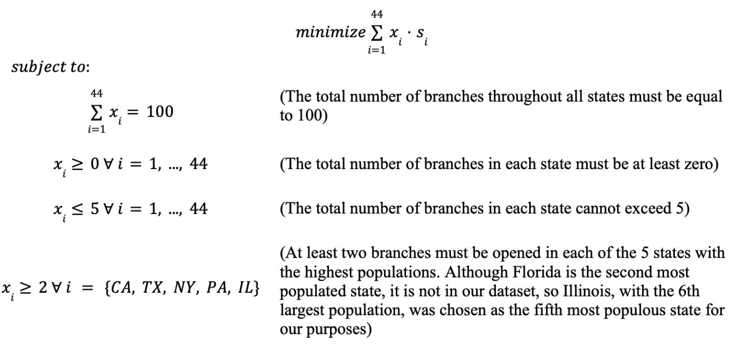
where
Below are the results of the prediction model minimizing the economic impact of natural disasters on the nationally expanding company:
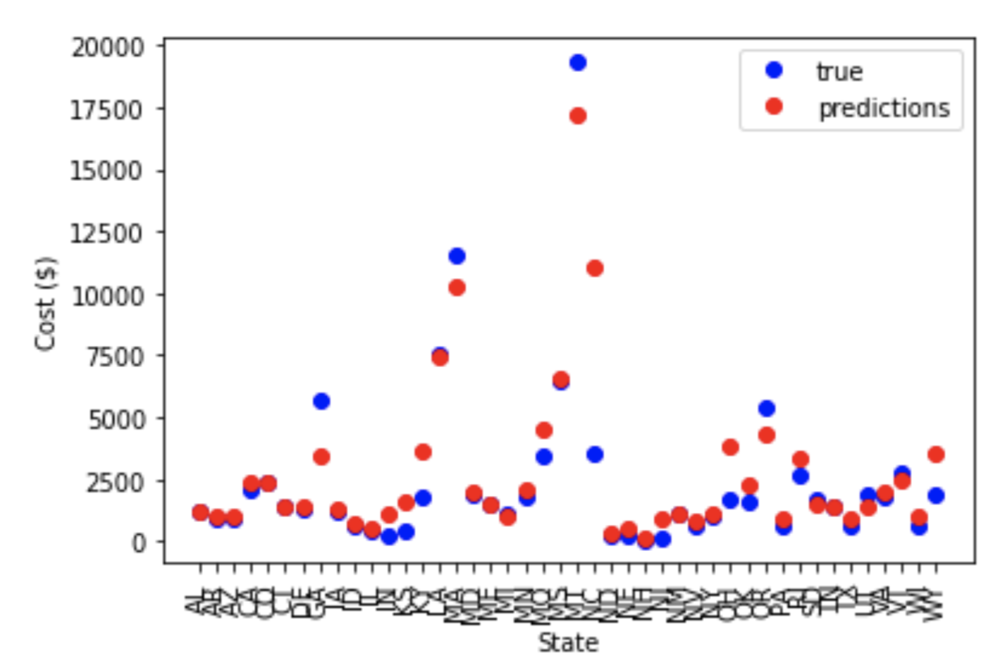
The average cost across all states is $2739.04 billion. The five states with the highest and lowest cost are detailed in the table below:
| Lowest Cost States | Highest Cost States | ||
|---|---|---|---|
| State | Cost ($ Billion) | State | Cost ($ Billion) |
| NH | 172.0416667 | MS | 6531.958333 |
| ND | 309.4166667 | LA | 7488.166667 |
| IL | 522.8333333 | MA | 10272.47917 |
| NE | 541.75 | NC | 11094.66667 |
| ID | 760.9166667 | MT | 17165.83333 |
The optimization model solved using "cvxpy" showed that 21 out of 44 states should have at least two branches opened in order to minimize economic loss for the company, while the remaining states had no branches opened.
| State | # Branches | State | # Branches | State | # Branches |
|---|---|---|---|---|---|
| AL | 5 | IL | 5 | NM | 5 |
| AR | 5 | IN | 5 | NV | 5 |
| AZ | 5 | MI | 5 | NY | 5 |
| CA | 2 | ND | 5 | PA | 5 |
| DE | 3 | NE | 5 | TX | 5 |
| IA | 5 | NH | 5 | UT | 5 |
| ID | 5 | NJ | 5 | WI | 5 |
To improve the prediction model:
- Gather more data across more years and more features
- Complete hyperparameter tuning using parallel computation or libraries such as optuna or hyperopt.
For the optimization model:
- Obtain additional datasets covering more attributes.
- Rerun the model with new constraints for a different branch distribution among states.