from os import listdir
from numpy import array
from keras.preprocessing.text import Tokenizer, one_hot
from keras.preprocessing.sequence import pad_sequences
from keras.models import Model
from keras.utils import to_categorical
from keras.layers import Embedding, TimeDistributed, RepeatVector, LSTM, concatenate , Input, Reshape, Dense, Flatten
from keras.preprocessing.image import array_to_img, img_to_array, load_img
from keras.applications.inception_resnet_v2 import InceptionResNetV2, preprocess_input
import numpy as np
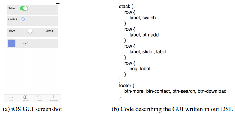
结合CNN与LSTM的方法,使用cnn抽取图像特征,使用RNN学习文本和序列规律,把两组上下文集成起来,我们就有信息知道一张设计图原型的语义,每个语义对应DSL,最后根据DSL生成源代码。
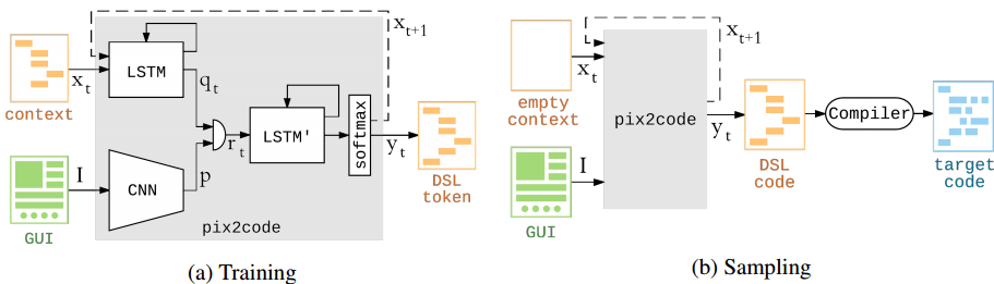
训练数据有两部分:
-
GUI原型图
-
DSL上下文
- 一个CNN网络来理解GUI内容,获得GUI图像特征。
- 一个LSTM网络来理解DSL上下文的基本规律,a单词token产生下一个b单词token的规律(不包含与原型图的关系) 两层各128个单元的LSTM模块
- 另一个LSTM‘ 用来理解DSL与对应原型图的关系,x原型图应该生成怎样的上下文token c? 两层各512个单元的LSTM模块
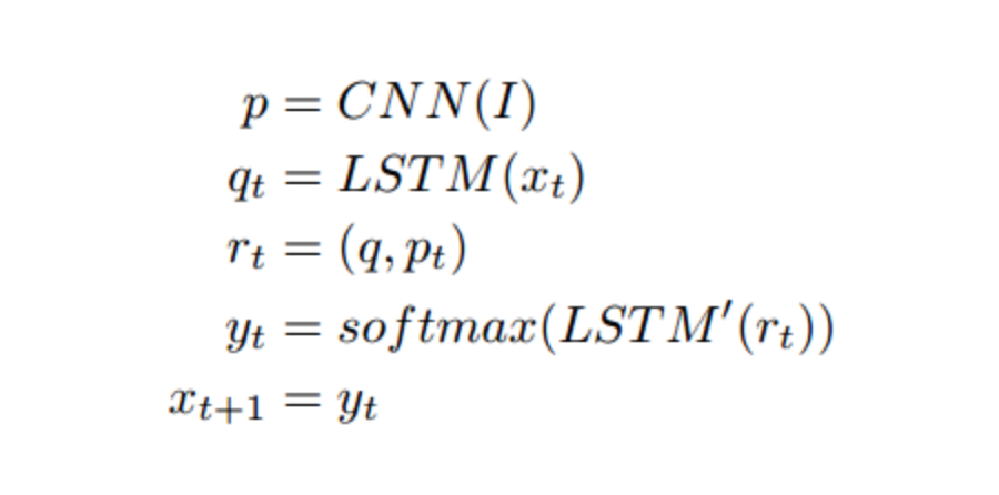
通过拼接cnn输出p和LSTM的隐层输出q,合成为r作为原型图和DSK相关性的依据。
最终的目标我们将通过手绘简笔画,生成视觉原型稿,再由对视觉原型稿生成dsl,通过对dsl生成各个平台android,ios,html代码。

"""
  准备图像特征数据

"""

# Load the images and preprocess them for inception-resnet
images = []
all_filenames = listdir('images/')
all_filenames.sort()
for filename in all_filenames:
    images.append(img_to_array(load_img('images/'+filename, target_size=(299, 299))))
images = np.array(images, dtype=float)
images = preprocess_input(images)

# Run the images through inception-resnet and extract the features without the classification layer
IR2 = InceptionResNetV2(weights='imagenet', include_top=False)
features = IR2.predict(images)在进行自然语言处理之前,需要对文本进行处理。 下面将介绍keras提供的预处理包keras.preproceing下的text与序列处理模块sequence模块。
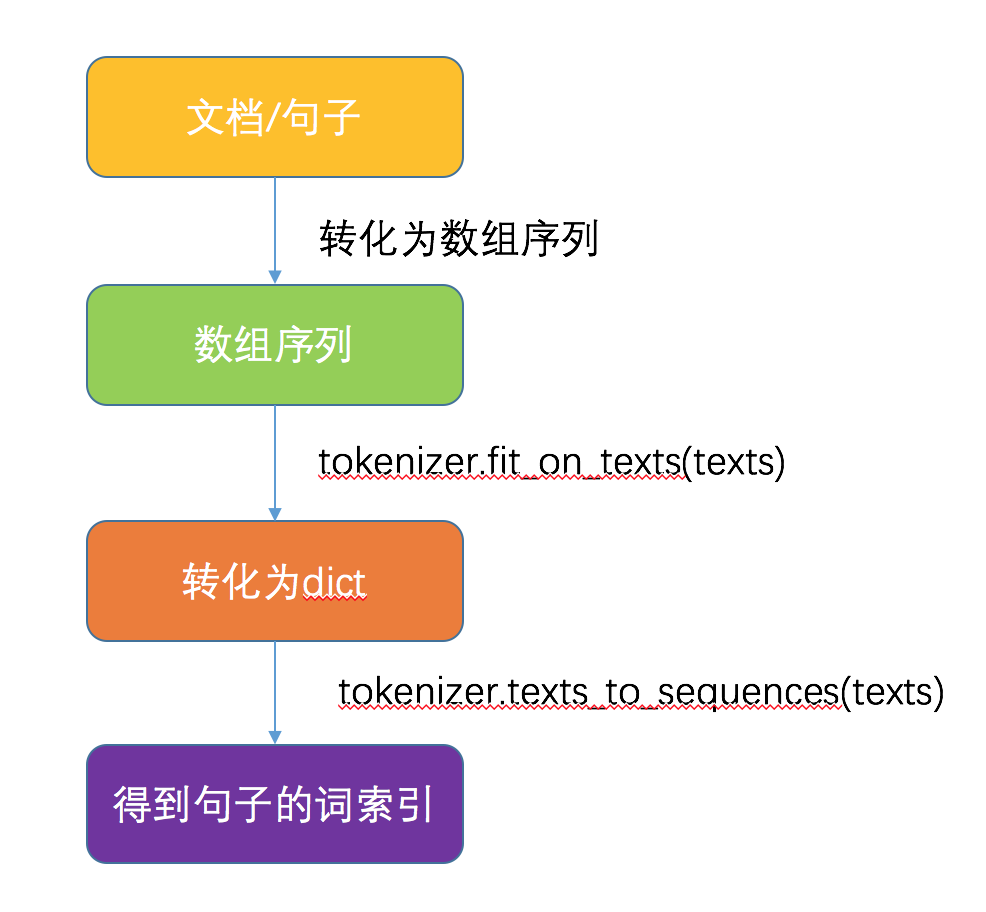
单词预处理的整体步骤如下:
- text_to_word_sequence(text,fileter) 可以简单理解此函数功能类str.split
- one_hot(text,vocab_size) 基于hash函数(桶大小为vocab_size),将一行文本转换向量表示(把单词数字化,vocab_size=5表示所有单词全都数字化在5以内)
这个类用来对文本中的词进行统计计数,生成文档词典,以支持基于词典位序生成文本的向量表示。 init(num_words) 构造函数,传入词典的最大值
- fit_on_text(texts) 使用一系列文档来生成token词典,texts为list类,每个元素为一个文档。
- texts_to_sequences(texts) 将多个文档转换为word下标的向量形式,shape为[len(texts),len(text)] -- (文档数,每条文档的长度)
- texts_to_matrix(texts) 将多个文档转换为矩阵表示,shape为[len(texts),num_words]
- document_count 处理的文档数量
- word_index 一个dict,保存所有word对应的编号id,从1开始
- word_counts 一个dict,保存每个word在所有文档中出现的次数
- word_docs 一个dict,保存每个word出现的文档的数量
- index_docs 一个dict,保存word的id出现的文档的数量
import keras.preprocessing.text as T
from keras.preprocessing.text import Tokenizer

text1='some thing to eat'
text2='some thing to drink'
texts=[text1,text2]

print T.text_to_word_sequence(text1)  #以空格区分,中文也不例外 ['some', 'thing', 'to', 'eat']
print T.one_hot(text1,10)  #[7, 9, 3, 4] -- (10表示数字化向量为10以内的数字)
print T.one_hot(text2,10)  #[7, 9, 3, 1]

tokenizer = Tokenizer(num_words=None) #num_words:None或整数,处理的最大单词数量。少于此数的单词丢掉
tokenizer.fit_on_texts(texts)
print( tokenizer.word_counts) #[('some', 2), ('thing', 2), ('to', 2), ('eat', 1), ('drink', 1)]
print( tokenizer.word_index) #{'some': 1, 'thing': 2,'to': 3 ','eat': 4, drink': 5}
print( tokenizer.word_docs) #{'some': 2, 'thing': 2, 'to': 2, 'drink': 1,  'eat': 1}
print( tokenizer.index_docs) #{1: 2, 2: 2, 3: 2, 4: 1, 5: 1}

# num_words=多少会影响下面的结果,行数=num_words
print( tokenizer.texts_to_sequences(texts)) #得到词索引[[1, 2, 3, 4], [1, 2, 3, 5]]
print( tokenizer.texts_to_matrix(texts))  # 矩阵化=one_hot
[[ 0.,  1.,  1.,  1.,  1.,  0.,  0.,  0.,  0.,  0.],
 [ 0.,  1.,  1.,  1.,  0.,  1.,  0.,  0.,  0.,  0.]]
embending层看这篇文档 http://frankchen.xyz/2017/12/18/How-to-Use-Word-Embedding-Layers-for-Deep-Learning-with-Keras/
"""
 对训练的code数据进行预处理
"""
# We will cap each input sequence to 100 tokens
max_caption_len = 100
# Initialize the function that will create our vocabulary
tokenizer = Tokenizer(filters='', split=" ", lower=False)

# Read a document and return a string
def load_doc(filename):
    file = open(filename, 'r')
    text = file.read()
    file.close()
    return text

# Load all the HTML files
X = []
all_filenames = listdir('html/')
all_filenames.sort()
for filename in all_filenames:
    X.append(load_doc('html/'+filename))

# Create the vocabulary from the html files
tokenizer.fit_on_texts(X)

# Add +1 to leave space for empty words
vocab_size = len(tokenizer.word_index) + 1
# Translate each word in text file to the matching vocabulary index
sequences = tokenizer.texts_to_sequences(X)
# The longest HTML file
max_length = max(len(s) for s in sequences)

# Intialize our final input to the model
X, y, image_data = list(), list(), list()
for img_no, seq in enumerate(sequences):
    for i in range(1, len(seq)):
        # Add the entire sequence to the input and only keep the next word for the output
        in_seq, out_seq = seq[:i], seq[i]
        # If the sentence is shorter than max_length, fill it up with empty words
        in_seq = pad_sequences([in_seq], maxlen=max_length)[0]
        # Map the output to one-hot encoding
        out_seq = to_categorical([out_seq], num_classes=vocab_size)[0]
        # Add and image corresponding to the HTML file
        image_data.append(features[img_no])
        # Cut the input sentence to 100 tokens, and add it to the input data
        X.append(in_seq[-100:])
        y.append(out_seq)

X, y, image_data = np.array(X), np.array(y), np.array(image_data)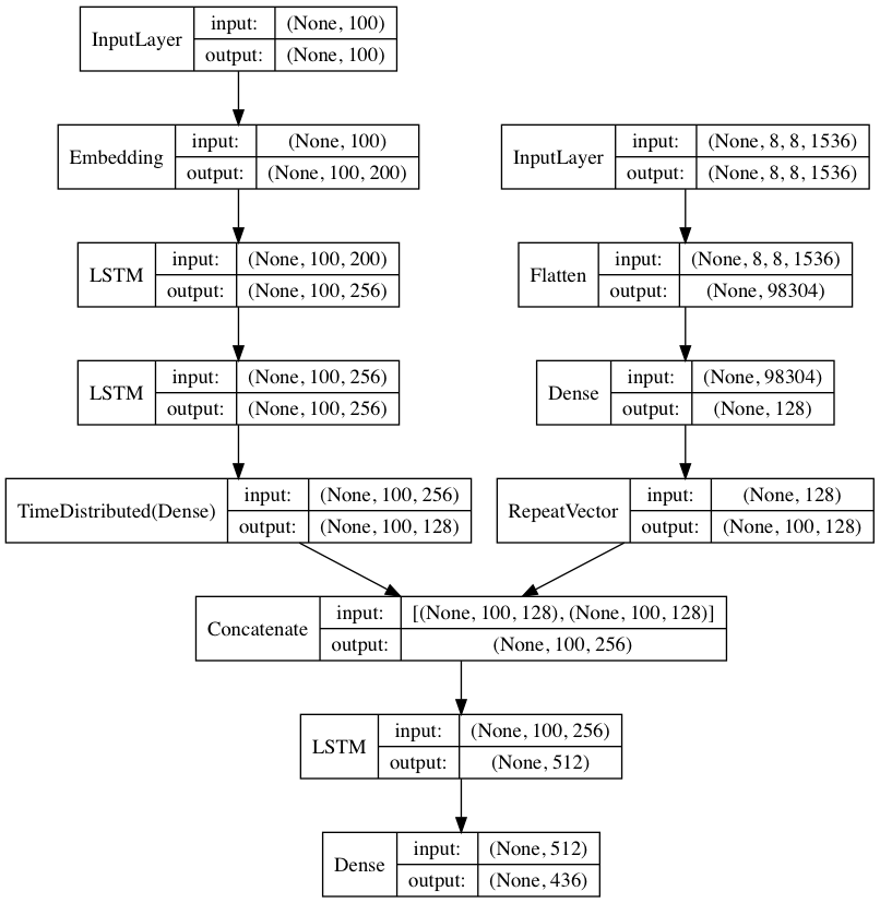
from keras.layers import Input, Dense
from keras.models import Model

# This returns a tensor
inputs = Input(shape=(784,))

# a layer instance is callable on a tensor, and returns a tensor
x = Dense(64, activation='relu')(inputs)
x = Dense(64, activation='relu')(x)
predictions = Dense(10, activation='softmax')(x)

# This creates a model that includes
# the Input layer and three Dense layers
model = Model(inputs=inputs, outputs=predictions)
model.compile(optimizer='rmsprop',
              loss='categorical_crossentropy',
              metrics=['accuracy'])
model.fit(data, labels)  # starts training
使用函数式模型的一个典型场景是搭建多输入、多输出的模型。
考虑这样一个模型。我们希望预测Twitter上一条新闻会被转发和点赞多少次。模型的主要输入是新闻本身,也就是一个词语的序列。但我们还可以拥有额外的输入,如新闻发布的日期等。这个模型的损失函数将由两部分组成,辅助的损失函数评估仅仅基于新闻本身做出预测的情况,主损失函数评估基于新闻和额外信息的预测的情况,即使来自主损失函数的梯度发生弥散,来自辅助损失函数的信息也能够训练Embeddding和LSTM层。在模型中早点使用主要的损失函数是对于深度网络的一个良好的正则方法。总而言之,该模型框图如下:
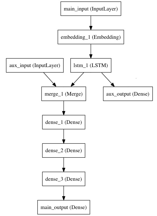
主要的输入接收新闻本身,即一个整数的序列(每个整数编码了一个词)。这些整数位于1到10,000之间(即我们的字典有10,000个词)。这个序列有100个单词。
from keras.layers import Input, Embedding, LSTM, Dense
from keras.models import Model

# Headline input: meant to receive sequences of 100 integers, between 1 and 10000.
# Note that we can name any layer by passing it a "name" argument.
main_input = Input(shape=(100,), dtype='int32', name='main_input')

# This embedding layer will encode the input sequence
# into a sequence of dense 512-dimensional vectors.
x = Embedding(output_dim=512, input_dim=10000, input_length=100)(main_input)

# A LSTM will transform the vector sequence into a single vector,
# containing information about the entire sequence
lstm_out = LSTM(32)(x)
然后,我们插入一个额外的损失,使得即使在主损失很高的情况下,LSTM和Embedding层也可以平滑的训练。
auxiliary_output = Dense(1, activation='sigmoid', name='aux_output')(lstm_out)
再然后,我们将LSTM与额外的输入数据串联起来组成输入,送入模型中:
auxiliary_input = Input(shape=(5,), name='aux_input')
x = keras.layers.concatenate([lstm_out, auxiliary_input])

# We stack a deep densely-connected network on top
x = Dense(64, activation='relu')(x)
x = Dense(64, activation='relu')(x)
x = Dense(64, activation='relu')(x)

# And finally we add the main logistic regression layer
main_output = Dense(1, activation='sigmoid', name='main_output')(x)
最后,我们定义整个2输入,2输出的模型:
model = Model(inputs=[main_input, auxiliary_input], outputs=[main_output, auxiliary_output])
模型定义完毕,下一步编译模型。我们给额外的损失赋0.2的权重。我们可以通过关键字参数loss_weights或loss来为不同的输出设置不同的损失函数或权值。这两个参数均可为Python的列表或字典。这里我们给loss传递单个损失函数,这个损失函数会被应用于所有输出上。
model.compile(optimizer='rmsprop', loss='binary_crossentropy',
              loss_weights=[1., 0.2])
编译完成后```,我们通过传递训练数据和目标值训练该模型:
epochs=50, batch_size=32)
"""
搭建代码生成网络
"""
'\n搭建代码生成网络\n'
# Create the encoder
image_features = Input(shape=(8, 8, 1536,))
image_flat = Flatten()(image_features)
image_flat = Dense(128, activation='relu')(image_flat)
ir2_out = RepeatVector(max_caption_len)(image_flat)

language_input = Input(shape=(max_caption_len,))
language_model = Embedding(vocab_size, 200, input_length=max_caption_len)(language_input)
language_model = LSTM(256, return_sequences=True)(language_model)
language_model = LSTM(256, return_sequences=True)(language_model)
language_model = TimeDistributed(Dense(128, activation='relu'))(language_model)

# Create the decoder
decoder = concatenate([ir2_out, language_model])
decoder = LSTM(512, return_sequences=False)(decoder)
decoder_output = Dense(vocab_size, activation='softmax')(decoder)

# Compile the model
model = Model(inputs=[image_features, language_input], outputs=decoder_output)
model.compile(loss='categorical_crossentropy', optimizer='rmsprop')
"""
epches代表训练轮次,训练次数越多,模型拟合的越好,尝试训练500次,最终的结果将非常好,
自己电脑估计得跑个一百天,还是得用GPU来跑,否则存在非常大的瓶颈
这里我就进行训练两次看下效果
"""
# Train the neural network
model.fit([image_data, X], y, batch_size=64, shuffle=False, epochs=500)Epoch 1/500
2306/2306 [==============================] - 74s 32ms/step - loss: 5.9631
Epoch 2/500
2306/2306 [==============================] - 56s 24ms/step - loss: 5.7329
Epoch 3/500
2306/2306 [==============================] - 53s 23ms/step - loss: 5.7348
Epoch 4/500
2306/2306 [==============================] - 53s 23ms/step - loss: 5.7193
Epoch 5/500
2306/2306 [==============================] - 56s 24ms/step - loss: 5.7287
Epoch 6/500
2306/2306 [==============================] - 56s 24ms/step - loss: 5.7258
Epoch 7/500
2306/2306 [==============================] - 52s 23ms/step - loss: 5.7222
Epoch 8/500
2306/2306 [==============================] - 52s 23ms/step - loss: 5.6982
Epoch 9/500
2306/2306 [==============================] - 53s 23ms/step - loss: 5.6962
Epoch 10/500
2306/2306 [==============================] - 53s 23ms/step - loss: 5.6940
Epoch 11/500
2306/2306 [==============================] - 53s 23ms/step - loss: 5.6632
Epoch 12/500
2306/2306 [==============================] - 52s 23ms/step - loss: 5.6747
Epoch 13/500
2306/2306 [==============================] - 55s 24ms/step - loss: 5.6520
Epoch 14/500
2306/2306 [==============================] - 56s 24ms/step - loss: 5.6181
Epoch 15/500
2306/2306 [==============================] - 62s 27ms/step - loss: 5.6160
Epoch 16/500
2306/2306 [==============================] - 73s 32ms/step - loss: 5.5654
Epoch 17/500
2306/2306 [==============================] - 73s 32ms/step - loss: 5.5521
Epoch 18/500
2306/2306 [==============================] - 71s 31ms/step - loss: 5.5783
Epoch 19/500
2306/2306 [==============================] - 67s 29ms/step - loss: 5.5496
Epoch 20/500
2306/2306 [==============================] - 56s 24ms/step - loss: 5.5791
Epoch 21/500
2306/2306 [==============================] - 52s 22ms/step - loss: 5.5695
Epoch 22/500
2306/2306 [==============================] - 52s 23ms/step - loss: 5.5415
Epoch 23/500
2306/2306 [==============================] - 53s 23ms/step - loss: 5.5227
Epoch 24/500
2306/2306 [==============================] - 54s 23ms/step - loss: 5.5116
Epoch 25/500
2306/2306 [==============================] - 53s 23ms/step - loss: 5.5102
Epoch 26/500
2306/2306 [==============================] - 55s 24ms/step - loss: 5.5112
Epoch 27/500
2306/2306 [==============================] - 71s 31ms/step - loss: 5.4835
Epoch 28/500
2306/2306 [==============================] - 70s 31ms/step - loss: 5.4915
Epoch 29/500
2306/2306 [==============================] - 71s 31ms/step - loss: 5.5190
Epoch 30/500
2306/2306 [==============================] - 69s 30ms/step - loss: 5.5060
Epoch 31/500
2306/2306 [==============================] - 69s 30ms/step - loss: 5.4695
Epoch 32/500
2306/2306 [==============================] - 54s 23ms/step - loss: 5.4543
Epoch 33/500
2306/2306 [==============================] - 55s 24ms/step - loss: 5.4532
Epoch 34/500
2306/2306 [==============================] - 57s 25ms/step - loss: 5.4398
Epoch 35/500
2306/2306 [==============================] - 58s 25ms/step - loss: 5.4521
Epoch 36/500
2306/2306 [==============================] - 75s 33ms/step - loss: 5.4576
Epoch 37/500
2306/2306 [==============================] - 75s 32ms/step - loss: 5.4074
Epoch 38/500
2306/2306 [==============================] - 269s 117ms/step - loss: 5.3958
Epoch 39/500
2306/2306 [==============================] - 74s 32ms/step - loss: 5.4328
Epoch 40/500
2306/2306 [==============================] - 79s 34ms/step - loss: 5.4458
Epoch 41/500
2306/2306 [==============================] - 77s 33ms/step - loss: 5.4608
Epoch 42/500
2306/2306 [==============================] - 74s 32ms/step - loss: 5.4334
Epoch 43/500
2306/2306 [==============================] - 67s 29ms/step - loss: 5.4661
Epoch 44/500
2306/2306 [==============================] - 66s 29ms/step - loss: 5.4235
Epoch 45/500
2306/2306 [==============================] - 53s 23ms/step - loss: 5.4088
Epoch 46/500
2306/2306 [==============================] - 51s 22ms/step - loss: 5.3967
Epoch 47/500
2306/2306 [==============================] - 52s 22ms/step - loss: 5.3826
Epoch 48/500
2306/2306 [==============================] - 50s 22ms/step - loss: 5.4172
Epoch 49/500
2306/2306 [==============================] - 51s 22ms/step - loss: 5.4210
Epoch 50/500
2306/2306 [==============================] - 52s 22ms/step - loss: 5.4141
Epoch 51/500
2306/2306 [==============================] - 51s 22ms/step - loss: 5.4013
Epoch 52/500
2306/2306 [==============================] - 51s 22ms/step - loss: 5.4160
Epoch 53/500
2306/2306 [==============================] - 50s 22ms/step - loss: 5.4031
Epoch 54/500
2306/2306 [==============================] - 52s 23ms/step - loss: 5.4265
Epoch 55/500
2306/2306 [==============================] - 53s 23ms/step - loss: 5.4474
Epoch 56/500
2306/2306 [==============================] - 51s 22ms/step - loss: 5.3995
Epoch 57/500
2306/2306 [==============================] - 52s 22ms/step - loss: 5.3882
Epoch 58/500
2306/2306 [==============================] - 74s 32ms/step - loss: 5.4082
Epoch 59/500
2306/2306 [==============================] - 57s 25ms/step - loss: 5.4277
Epoch 60/500
2306/2306 [==============================] - 54s 23ms/step - loss: 5.4727
Epoch 61/500
2306/2306 [==============================] - 58s 25ms/step - loss: 5.4171
Epoch 62/500
2306/2306 [==============================] - 61s 27ms/step - loss: 5.3906
Epoch 63/500
2306/2306 [==============================] - 57s 25ms/step - loss: 5.4031
Epoch 64/500
2306/2306 [==============================] - 61s 26ms/step - loss: 5.3931
Epoch 65/500
2306/2306 [==============================] - 75s 33ms/step - loss: 5.3620
Epoch 66/500
2306/2306 [==============================] - 71s 31ms/step - loss: 5.4000
Epoch 67/500
2306/2306 [==============================] - 71s 31ms/step - loss: 5.3857
Epoch 68/500
2306/2306 [==============================] - 74s 32ms/step - loss: 5.3546
Epoch 69/500
2306/2306 [==============================] - 71s 31ms/step - loss: 5.3431
Epoch 70/500
2306/2306 [==============================] - 70s 30ms/step - loss: 5.3481
Epoch 71/500
2306/2306 [==============================] - 75s 33ms/step - loss: 5.3435
Epoch 72/500
2306/2306 [==============================] - 71s 31ms/step - loss: 5.3395
Epoch 73/500
384/2306 [===>..........................] - ETA: 1:06 - loss: 5.2904
# map an integer to a word
def word_for_id(integer, tokenizer):
    for word, index in tokenizer.word_index.items():
        if index == integer:
            return word
    return None
# generate a description for an image
def generate_desc(model, tokenizer, photo, max_length):
# seed the generation process
in_text = 'START'
# iterate over the whole length of the sequence
for i in range(900):
# integer encode input sequence
sequence = tokenizer.texts_to_sequences([in_text])[0][-100:]
# pad input
sequence = pad_sequences([sequence], maxlen=max_length)
# predict next word
yhat = model.predict([photo,sequence], verbose=0)
# convert probability to integer
yhat = np.argmax(yhat)
# map integer to word
word = word_for_id(yhat, tokenizer)
# stop if we cannot map the word
if word is None:
break
# append as input for generating the next word
in_text += ' ' + word
# Print the prediction
print(' ' + word, end='')
# stop if we predict the end of the sequence
if word == 'END':
break
return# Load and image, preprocess it for IR2, extract features and generate the HTML
test_image = img_to_array(load_img('images/87.jpg', target_size=(299, 299)))
test_image = np.array(test_image, dtype=float)
test_image = preprocess_input(test_image)
test_features = IR2.predict(np.array([test_image]))
generate_desc(model, tokenizer, np.array(test_features), 100)